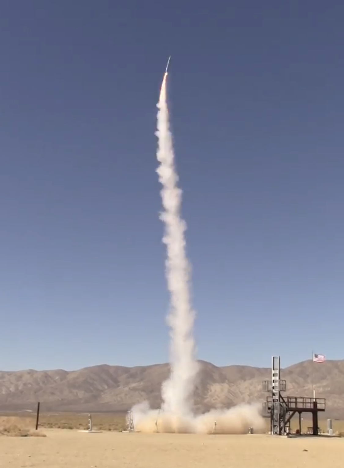
RRS member, Bill Claybaugh, built and launched his second 6-inch rocket from the RRS Mojave Test Area on Saturday, April 22, 2023. Target apogee was 69,000 feet. Winds were very low that day. Jim Gross was the pyrotechnic operator in charge for the launch event. Dimitri Timohovich and Rushd Julfiker assisted with the efforts. Bill launched from a 24-foot aluminum channel type launch rail using a pair of belly-bands that disconnected from the vehicle after clearing the end of the rail. The following is Bill’s update report on the flight as of July 1, 2023.
Flight 2 –Six Inch Rocket
Fight II Flight Report
Introduction
Something fairly violent happen to this vehicle at about 3.4 seconds into flight: onboard data and ground video indicate the rocket pitched at least 30 degrees while traveling at about Mach 2.2 at around 4100 feet above ground level (AGL).
Recovered hardware indicates the vehicle broke up under these conditions. The parachute compartment, which was attached to the top of the motor by four ¼-20 fasteners, was torn away by fracture at all four fasteners (the fasteners remained attached to the motor). The payload, which was attached to the parachute compartment via four 0.250” diameter pneumatic separation system pins, remained attached—indeed, it was recovered with the separation system still functional and still latched to the top of the parachute compartment.
Bill Claybaugh with his second 6-inch rocket before launch.
Video shows a sudden pitch at about 3.4 seconds after first vehicle motion. The onboard data (which records the initial part of the breakup because the computer was located in the payload section) shows that the gyro tilt went from about 5 degrees to 50 degrees over 0.08 seconds. Measured longitudinal acceleration went from the previous around 26 g’s to 34 g’s in 0.05 seconds, and after returning to around 24 g’s for 0.15 seconds, to -12.7 g’s (the sensor floor) for 0.03 seconds, before recovering to -9 g’s for 0.01 seconds followed by loss of power. (See Chart 1.)
Chart 1: Acceleration and Tilt
Video shows the vehicle recovering from this pitch maneuver and continuing on a near vertical ascent though burnout at a video-based about nine seconds after first motion.
Flight
Following failure of the AlClO (Aluminum / Potassium Perchlorate) based head end initiator to successfully ignite the rocket (AlClO based initiators have had this issue previously, AlClO appears to be too energetic for this application, tending to blow the secondary ignition materials out the back of the rocket and on to the ground rather than igniting the grain) a jury-rigged rear end ignitor was substituted and the rocket successfully lifted off about 0.25 seconds after flames first appeared around the vehicle base.
Onboard data shows the vehicle ascending at about 88 degrees from horizontal to about 50 feet altitude when a lazy “S” turn (first to the northeast, then back to the southwest) is visible in the video and data. This turn starts about the time the belly-bands can be seen on video falling away from the vehicle.
Following this maneuver, the vehicle returns to near vertical flight to the Southwest, turning, with perturbations, from about 88 degrees tilt to an 86-degree gyro tilt over the next two-plus seconds. Acceleration steadily builds from an initial 18.6 g’s to a maximum of 27.3 g’s at 2.53 seconds; this acceleration broadly follows the curve expected from the combination of the thrust curve, drag, and the lessening weight of the vehicle as propellant is consumed, however, the measured acceleration is much higher than expected based on static tests and flight simulations.
Telemetry reported Loss of Signal (LOS) at 2.7 seconds and at an (accelerometer-based) 2313 feet altitude and 2440 ft/sec velocity.
Measured onboard acceleration suddenly jumps from a base around 26.5 g’s at 3.18 seconds to 32.8 g’s at 3.21 seconds; measured onboard acceleration stays above 30g’g for the next 0.06 seconds, peaking at 34.7 g’s at 3.21 seconds and followed by a return to around 24 g’s for 0.15 seconds and a sudden drop to -12.7 g’s (the sensor floor) from 3.42 to 3.44 seconds and a final reading of -9.3 g’s followed by loss of power to the on-board computer.
Onboard data shows the gyro tilt angle moving from around 5 degrees at 3.37 seconds to 50.6 degrees at 3.45 seconds, followed by loss of power.
Video over this period show the vehicle suddenly turning through an apparent (visual) 30 degrees or so before pitching back to a near vertical ascent.
Analysis
A less energetic initiator is required for this vehicle; a development program will be initiated to achieve both a more reliable and a gentler ignition in future.
Figutr 1: Recovered Nozzle
Following flight, a single sliver of graphite was found on the ground about 150 feet from the launch tower. This piece of graphite was exactly the correct shape to fit at the very rear of the graphite throat insert where that insert blends into the titanium nozzle extension.
Recovered nozzle hardware showed that about 1-inch of the rear of the nozzle insert was missing (see Image 1); assuming the two pieces of the insert found inside the rocket were broken by impact forces, it follows that around one inch at the rear of the insert failed prior to impact. This failure would have induced a flow discontinuity in the rocket’s exhaust which thrust vector could account for the sudden pitch at 3.4 seconds into flight. The vehicle’s return to near vertical ascent appears to be due to aerodynamic assisted dampening of the perturbation, based on the tilt data from the earlier–possibly belly-band related–slow spiral of the vehicle.
Note that the recovered nozzle shows plating of Aluminum Oxide onto the ZrO coated Titanium nozzle extension above the end of the graphite nozzle extension but not in the area originally covered by the graphite insert. This suggests the insert was present during startup (when Aluminum Oxide would be expected to condense on the nozzle extension surface) and the loss of the about 1-inch of the bottom of the graphite nozzle insert must have occurred later.
Analysis indicates that thermal stress cannot have been the cause of the loss of the back of the nozzle insert: maximum thermal stress occurs at the throat and reaches no more than 60% of the tensile strength of the graphite. Careful measurement shows that the break occurred at the location of the joint between the titanium nozzle extension and the aluminum nozzle support structure, it thus appears that a (possibly heating related) stress concentration at that location was the probable cause of the graphite failure.
Loss of telemetry at 2.7 seconds appears to be a consequence of the GPS and transmitter antenna assembly failing mechanically; the flight computer was recovered with a clean break at the antenna PCB board. This suggests the need for more robust support of these parts of the payload.
Breakup of the vehicle began about 3.41 seconds after launch. The recovered pieces indicate separation of the parachute compartment from the motor was due to the upper part of the vehicle being pulled longitudinally forward, away from the (thrusting) rocket motor; further, the fracture pattern indicates an abrupt failure rather than a slightly slower swaging of the metal. Based on the acceleration data indicating at least four hundredths of a second of significant negative g’s just before loss of power, coupled with gyro data showing the payload being thrown through an about 45 degree turn over the last 0.08 seconds of data, we can guess that the mechanical failure was a consequence of rather than the cause of the sudden turn of the vehicle.
Figure 2: Booster, post-impact
Actions
Development of a gentler and more consistent initiator is required; an effort focused on BKNO3/V (Potassium Nitrate with Boron held in a Viton matrix) has been started.
The vehicle nozzle has been redesigned to use a single piece titanium throat insert support structure and nozzle extension. The angle of the joint between the graphite insert and the titanium shell has been increased to the conventional 5 degrees (the flight nozzle used a 3-degree angle that may have been too thin at the very end of the throat insert).
Heat paint testing of the Titanium nozzle extension on the flight nozzle indicated a maximum heat soak temperature of about 800° degrees Fahrenheit on the outside surface; this suggests a maximum outside wall temperature during operation of about one-half the paint-indicated heat-soaked temperature. Since these temperatures are well below the maximum working temperature of 6Al4V Titanium under these loads, the new nozzle is designed to allow for greater heating of the shell.
Analysis based on assuming a maximum Titanium temperature during operation of about 400° F indicates a maximum possible temperature of about 1140° degrees at the ZrO / Titanium interface and about 2800 °F at the inside surface of the Graphite insert, implying a maximum surface temperature at the nozzle throat of about 4350 °F. A similar analysis indicates a maximum possible temperature at the inside surface of the nozzle exit of about 3300° F.
The high temperature RTV layer between the graphite insert and the ZrO layer was originally 0.005” in thickness in two sections separated by a 0.030” cork layer (a total of 0.010” of RTV); it thus should have had sufficient space, after pyrolysis of that layer, to accommodate the estimated 0.0024” thermal expansion of the Graphite Nozzle Insert.
The payload internal fiberglass support structure for the flight computer failed both at the base and at the antennae. This structure will be redesigned in aluminum so as to provide still more robust support to the flight computer assembly. Making this change will reduce the sensitivity of the GPS antenna and will absorb some of the transmitted energy from the telemetry antenna (the reason for going with fiberglass previously). The effects of lower sensitivity will have to documented once that hardware is available and assembled.
The measured inflight acceleration is significantly higher than that expected from static testing and modeling of the flight trajectory; however, the burn time indicated from multiple videos is about that expected from motor modeling and the previous static test.
Analysis of the cause of the apparently higher than expected thrust has proven inconclusive. A grain crack or void (possibly associated with the energetic AlClO initiator) would usually be expected to grow until the motor case failed. The slightly higher than modeled initial grain area (see the report from the first flight of this vehicle for a discussion) is too small (at 0.86%) to account for the higher initial thrust (123% of the expected level). A static test motor is being prepared to try and resolve this question.
Strengthening the joint between the motor and the parachute compartment is relatively easy; additional fasteners and a thicker section to the joint should reduce the probability of a failure similar to that which occurred on this flight. Alternatively, the motor tube could be extended by six inches to avoid having a separate parachute compartment altogether, albeit with some induced operational inconvenience when placing the initiator into the forward bulkhead.
Summary
Partial nozzle failure appears to be the main concern with this vehicle design; a secondary issue is strengthening internal components and some joints to better survive the extremely harsh conditions encountered on this flight. Finally, a cause for the apparently higher initial thrust will be sought via static testing of a new motor, which will also confirm the new nozzle design.
I would like to set the record straight on a common mistake I see with designing parabolic rocket nozzles.
The simplest and most common nozzle used in amateur rocketry is the simple cone. Most commonly the cone is a 15° half angle. But the simplicity of the cone comes at the cost of reduced performance and increased length. The next step up in complexity is a parabolic bell nozzle.
The parabolic bell nozzle design is a little more complicated and much more difficult to manufacture. Machining a parabolic shape out of metal on a lathe by hand is doable with a digital read-out (DRO) device but the process would likely be very tedious. In this case, I would recommend looking into some sort of computer-controlled system like CNC or 3D printing. If you’re using an ablative composite like silica-phenolic then tuning a wood mandrel on a lathe is very doable. Beyond the parabolic nozzle the next step up in complexity and efficiency is using the method of characteristics to design a rocket nozzle. This method was pioneered by Gadicharla V.R. Rao.
.These are sometimes called “Rao” nozzles. The parabolic nozzle is a decent approximation of a Rao nozzle, a method also proposed by Rao. Going further to get the last drop of performance would require a detailed computational fluid dynamics (CFD) based optimization.
I’m writing this report to set the record straight on a common mistake I see with determining the proper geometric and dimensional features of specific parabolic rocket nozzles. Almost all the amateur parabolic nozzles I’ve seen up to this point, including several college teams, and even my own early designs, made this mistake. It’s not really their fault though. The parabolic nozzle is commonly mention in rocket literature but rarely is one particular key fact needed to make them correctly explained. The two of the most prolific textbooks on the topic are, “Rocket Propulsion Elements” by Sutton and Biblarz, and “Modern Engineering for Design of Liquid-Propellant Rocket Engines” by Huzel and Huang. Both give their readers charts to help design the parabola and both also neglect to mention this one important fact.
That there is a problem at all will only become apparent when you try to solve for the exact equation of the parabola. If you read through the common literature (a task left to the reader) and go through the process you will see that the parabola is defined by two points and two angles. The two points are the beginning and the ends of the parabola. The beginning point is where the curvature at the throat, typically a circular arc, transitions into the parabola. The end point is the exit of the nozzle. The two angles, θn at the beginning of the parabola and θe at the exit are the angles between the centerline of the nozzle and lines tangent to the parabola at the two points. These angles are normally found by using graphs given in the literature. These graphs are the angles vs expansion area ratio as shown below. Note that they present the length of the bell nozzle as a percentage, Lf, of the length of an equivalent conical nozzle with the same nozzle expansion area ratio and a 15° half angle.
Graph of theta angles from Rao’s paper
Footnote about the θn and θe vs expansion area ratio graphs.
I’d like to note that the graph I shared is the in the commonly presented form. However, if you look at the original paper on parabolic nozzles “Approximation of Optimum Thrust Nozzle Contour” by G.V.R. Rao in 1960” you will find the information presented differently. Instead of theta versus epsilon at various percentages of nozzle lengths given in terms of the percentage of an equivalent 15° conical nozzle length of the same expansion ratio (epsilon), the axes of graph are in terms of the ratios re/rt versus Ln/rt given at various values of θn and θe. These lines are straight in comparison to the curved lines in the graph above. The more common graphs are supposed to have been derived from the originals.
However, I have not gone through the math myself, but, I am interested in what the process and results would be. In turn, the originals are supposed to have been derived from full calculations of the Rao method. Again, something I have not tried replicating but it is something I would be interested in seeing the details of.
Another thing worth mentioning is that I recall reading online that someone had tried to reproduce these results using the method of characteristics. (Unfortunately, I cannot recall exactly where I read this.) The original graphs were based on using a fixed specific heat ratio (gamma) of γ=1.23 and the original paper stated “A different value of γ does not appear to appreciably change the nozzle contour when the area ratio and length are prescribed.” however the testimony I found online stated that they found that the gamma value did significantly affect the angles. I am in doubt over this anonymous internet testimony, but it is something I’m interested in exploring in more detail. If you ever investigate this yourself, dear reader, be sure to send us what you discover.
In total, you will have six parameters to determine, at point 1 you will have x1, y1, and θn. At point 2, you will have x2, y2, and θe. The obvious route from here would be to take the equation of a parabola (more precisely a square root since the x-axis will be our chamber centerline. But hey, a square root is just a parabola on its side), and these six parameters and try to solve for the unknowns in the equation.
This is where you run into the problem. The parabola is over-defined! You can’t solve for a parabola that meets all six criteria. It is impossible. Five of the defining parameters can be correct, but at least one will always be wrong. This is where most people, after considerable effort and eventually the banging of one’s head against a wall, will give up and let one, or more, of the 6 parameters to be wrong, usually by letting the starting angle of the parabola to be wrong.
When plotting a nozzle contour most put the centerline of the nozzle along the x-axis. The mistake everyone makes, including myself, is to make the natural assumption that this parabola is aligned with the nozzle’s same x and y axis in the same way as all of the parabolas in your algebra classes. That is to say the centerline of the parabola is around the x axis, the same axis of axial symmetry as the nozzle. But what everyone misses, including in the common literature, is that the parabola should be canted! That is to say, it should be rotated by some angle in relation to the x and y axis.
The way I found this fact out is by being a prolific reader. I’ve spent a lot of time gathering papers and books on rockets. I’ve only ever found one source that explicitly states the nature of these parabolasand that is in “Liquid Rocket Engine Nozzles NASA SP-8120” It simply refers the them as a “canted-parabola contour” and offers no further explanation. But that clue was enough for me to figure out what was going on. Adding the rotation of parabola adds a degree of freedom in the math. This allows for the equations to be solved with all the required constraints.
* Footnote on the NASA SP-8000 publication.
By the way, the NASA SP-8000 series of publications is a fantastic resource for the aspiring rocket scientist. Back in the 1970’s, they tried to write a comprehensive review of the state of the art in rockets and spaceflight. I remember reading somewhere that they fell short of their goal, since there was too much know-how to catalog. But what they did manage to publish is great. Whenever diving into an unfamiliar design topic, I’ll read the relevant SP-8000 article on it first as a good overview. Some topics may be more outdated than others, but much of it is still great and relevant today.
When trying figure this out, I went digging and found the original paper on parabolic nozzles. “Approximation of Optimum Thrust Nozzle Contour, by G.V.R. Rao, 1960” I had hoped it would directly state the parabola should be canted, but it doesn’t. However, it does give enough information to deduce this conclusion. In the short paper, its one page, Rao describes “a simple geometric construction for the parabolic contour.” It is something that would have been more familiar with the designers and draftsmen of that time. Today, we are more likely use a series of points and connect them with a spline curve, or use mathematical equations in CAD software to draw similar curves. But back then, designers would have to do it by hand on paper. The method suggested by Rao is called the “tangent method” of drawing a parabola. As the name suggests it involves drawing a series of lines that are tangent to the parabola.
Since we are interested in the mathematical equations, I won’t be describing that method any further. But it is plain to see from figures that the method does not directly depend upon the x, and y axis. The contour is simply plotted on the x-y plane and then the contour is revolved around to x-axis to create the three-dimensional nozzle. Since we cannot fit the desired parabola with the normal parabolic equations, we are left with the question:
How does one mathematically rotate the equation of a parabola?
Using parametric equations is how we will be able to create aparabola rotated on the x-y plane. Parametric equations also make some of the math easier when solving for circular arcs that are used in the rest of the nozzle contour.
First let’s start with vertex form a parabola.
Equation 1; vertex form of the parabola equation
To parameterize this, let us set:
Equation 2: parameterization or variable substitution
And solve for x and y.
Equations 3.1 and 3.2: Solving for x and y variables
This pair of equations is now a parametric form of a parabola. But it is just a regular parabola and we need to rotate it. Recall from your study of trigonometry, that the formulas for rotating a point around the origin by angle θ are:
Equations 4.1 and 4.2: Rotating the frame of reference by angle, theta
We can combine equations 3 and 4 by substituting the parametric equations into the place of x0 and y0. Doing this, we get:
Equations 5.1 amd 5.2: Combining prior equations 3 and 4
From this, we can get:
Equations 6.1 and 6.2: further derivation of x and y equations
Note that for our use case, because the rotation angle θ is a constant, h∙cosθ-k∙sinθ and h∙sinθ+k∙cosθ are also constants and can be replaced by single terms, c1 and c2 respectively. But we can name c1 and c2 whatever we like so I shall name them h and k respectively. (Yes, I know this seems like an odd maneuver, but it works fine for us and makes our equations a bit simpler.) With a little rearranging this then gives us the parametric form of a rotated parabola:
Equations 7.1 and 7.2: rearranging equations 6.1 and 6.2
Now we are ready to solve for the parabolic nozzle contour. Before we do this for the above equations, we shall discus the rest of the contour as well. We will use a piecewise set of equations to describe the entire contour. For each piece we will need to solve for parameters and the split points between the different pieces of the function. We will go through each of them in order. How to size a thrust chamber is beyond the scope of this paper and is an exercise left to the reader. You should already have calculated the radius of the chamber, throat, and nozzle exit, rc, rt, and re, respectively and the length of the chamber and nozzle, Lc, and Ln respectively. The figure below shows a typical form of a thrust chamber. You’ll note that I’ve used z and r instead of x and y. This is a notation that I adopted early in my work writing a code for thrust chamber design. I figured z is up and rockets go up, so that’s where I’ll put the axis of symmetry of the chamber. I put the throat at z=0 for convenience. I decided to keep my notation in this report, instead of adopting something more conventional, for my own convenience of not having to rewrite all of my equations.
CAD drawing of nozzle geometry with refernce points and radii, note the parabola axis is canted
The first part of our piecewise function f1 is the chamber section representing by red in the figure. f1 is a simple horizontal line with the equation.
f1 Chamber Section
Equation 8 descrbing the straight chamber section before the converging section that follows
f2 Concave Curved Converging Section
The exact converging section shape typically does not strongly affect engine performance. So, the designer has a lot of freedom here butthe following geometric convention is common. Three parts are used, f2 (blue in figure) is a concave circular arc, followed by f3(green in the figure) is sloped line and f4 (orange in the figure) is convex circular arc. I’ve found that using the parametric form of a circle makes the math easier. The parametric form of this circular arcin function 2 is the following.
Equation 9.1 amd 9.2 for a concave-type converging section
Were rf2 is the radius of curvature for function 2.
f3 Linear Converging Section
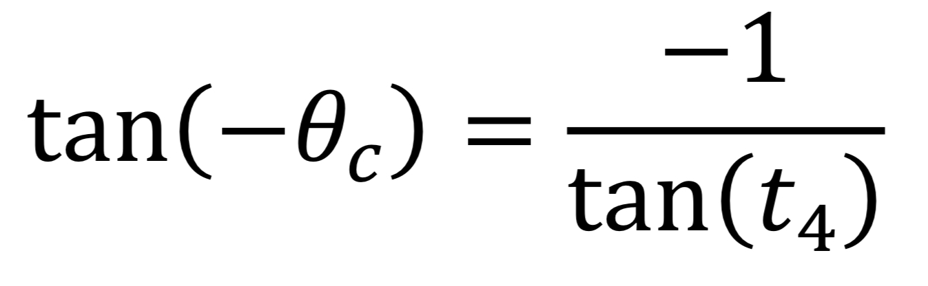
The third piece is a straight line and we will use the point slope formof a line. The designer provides the converging angle and a typical rule of thumb value is 30°. Using a bit of trigonometry, we can see that the slope will be tan(-θc). For the point we will use (z4, r4) which is where f3 intersects f4.
Equation 10: linear converging nozzle
f4 Convex Curved Converging Throat Section
The fourth piece is another circular arc. The radius of curvature is typically given by the designer as a multiple of the throat radius. A typical a rule of thumb value of 1.5 time the throat radius is commonly used. We will call this scalar rc2. Again, we will use the parametric form.
Equation 11: convex curved converging section
About solving for the unknowns upstream of the nozzle throat
Solving the converging section is where we will notice a hiccup (minor problem). Say that you have a large throat and a small contraction ratio, Ac/At. This could mean the point where f4 meets the given converging angle, θc, of f3, could be equal to or larger than the chamber radius. A mathematical solution that uses the given parameters would fail to produce real geometry. A second problem could arise even when a valid solution does exist because the result could be an undesirably sharp radius if the point is too close to the chamber radius.
So, we have two solution paths. For the conventional case, we don’t run into the previously mentioned hiccup. Here, functions f1, f3, and f4 are sufficiently defined by the given parameters mentioned so far. But to define where the function f2 is located, we will need an additional parameter. In my work, I’ve decided to do this by setting the point r3 to be a percentage of the vertical distance between the chamber radius and r4. Where the concave f2 curve meets the linear converging portion, f3, is the location of r3. Where f3 meets the convex f4 curve is r4. My default value is 50% of the way between r4 and rc. I’ve named that parameter f2vp and its value should be between 0 and 1. The letters used mean: function 2, vertical percentage. (You are probably asking yourself “Why not just define rf2 in the same way as rf4, with a scaler multiple of rt?” Well good question. That’s the way I started doing it. It’s been a while but if I remember correctly, I found that it was hard to pick a default value that worked for a large variety of engines and if picked poorly results were either undesirable or didn’t solve. So, I came up with the above method which I found much more satisfactory.)
For the second solution path an alternat method for defining the converging section must be used. It will be convenient to set the radius of both of the concave, f2, and convex, f4, sections equal. Then we define the curved converging sections, f2 and f4, to each take up a percentage of the radial distance between the throat and the chamber radius. The linear section is the remaining percentage. I’ve named this parameter f2vp_alt. The name means: function 2, vertical percentage alternate method. Since there are 3 functions that take up this vertical distance, and two of them are equal the value for f2vp_alt must be between 0 and 0.5. If it is 0 that means that the linear portion takes up all the vertical distance and the curved portions would disappear. If it is 0.5 then the linear portion would disappear. The default vale I use is 1/3. This means that f2 takes up 1/3 of the distance, and f4 takes up 1/3 of the distance and the linear section, f3, takes up the remaining 1/3. It makes for decent looking converging contours.
This will always be solvable with real geometry, but means that theeither the converging angle or the radius of curvature for the converging portions cannot be pre-defined and is instead solved for. At first, I tried to let the converging angle, θc be derived. However sometimes the solution would be a very shallow angle creating an overly long converging section. Instead, I found better results by keeping the designer given θc and instead solve for the radius of rf2and rf4, which would still be kept equal. I was resistant to this at first because it would remove the ability to use the rule of thumb value for rf4, or any specified value for that matter. This will only work if the assumption that the designer will provide reasonable values for θcis met. To summarize, the primary method lets the radius of function 2, rf2, be an unknown to be solved for, and the converging angle of f3is given and the radius of f4 is given. With the alternate method the converging angle is given along with the vertical space the functions occupy. This leaves the radiuses of curvature rf2 and rf4, which are equal, to be solved fore.
When I have designed thrust chambers, I use the first method and then only switch to the second method if the first method does not work. The remaining question is when to switch to avoid a sharp corner. My solution was to specify that the concave radius, f2, take up a minimum percentage of the vertical distance between the throatand chamber radius. My default value for this is 15% but this was somewhat arbitrary. You can also avoid the second method by increasing the thrust chamber contraction area ratio if possible.
Converging section solution, Method 1
The following is a mathematical solution for the converging section when using the regular method for the converging section described above. From f4 we need to solve for z4 and its corresponding radial point r4. For that we need to find when the circular arc is at the givenconverging angle. This is when its derivative is equal to the slope of f3, the linear section, which is tan(-θc). We will take the derivative ofthe parametric equations of function 4. In case you forgot from your calculus class the derivative of a parametric equation is found by taking the derivative of each equation separately with respect to the parametric independent variable, in this case t, which will give us the equations for and . Then you divide the equation for by the equation for and cancels out and you are left with an equation for . Using this method on the equations 11.1 and 11.2 for function 4 we get
Equation 12:
We solve this at t4 by setting the derivative equal to tan(-θc) which gives us
Equation 13:
Solving for t4 we get
Equation 14:
Note that this solution is periotic so it mathematically solves with any added to it. Through quick trial and error, we find a value n=1will put point (z4, r4) in the correct quadrant on the x-y plane. We then plug t4 into f4 to get the z4 and r4 coordinates.
Equations 15.1 and 15.2:
Now that we know that value of r4 we can now check if the criteria needed for switching to the alternate method is met. If not, we can carry on to find r3. Recalling our assertion that r3 shall be some given fraction of the vertical distance between r4 and rc we see that it would be given by the following equation.
Equation 16:
Next, we plug r3 into the f3 function [eq 10] and solve to get z3.
Equation 17:
Now all that remains to be solved is z2 and the radius of curvature, rf2, for the concaved converging function f2. If we take f2 [equation 9] and plug in the known point z3, and r3, which both occur at t3, we get the following:
Equation 18.1 and 18.2:
We can see that the there are three unknowns z2, rf2, and t3, but there are only two equations. So, we need a third equation to solve this system. We know the derivative of this function is the same as for the function f4, [equation12] since they are both the equations of a circle. And we know the value of the derivative at this intersection pointfrom the slope of f3, the linear converging section, which is tan(-θc).Setting equation 12 to tan(-θc) gives us the third equation we need.
Equation 19:
We then solve this system of three equations, 18.1, 18.2, and 19 for the three unknows z2, rf2, and t3. This gives us:
Equation 20:Equation 21:Equation 22:
We now have all the parameters and split points needed for each of the function to fully define the converging section. Equation 20 like in equation 14 also has a periodic portion of the solution, but here n=0.
Converging section solution, Method 2
With the second method everything is the same as the first method up to calculating t4 [equation 14] then the methods diverge. In method 2, after calculating t4 the next things to calculate are r3 and r4. This method defines the percentage of the radial distance between the throat and the chamber that the two curved converging functions, f2and f4, take up. This definition allows us to create, by reasoning, the equations for r3 and r4. They are:
Equation 23:Equation 24:
Next the radius rf4 can be found by taking f4r [equation 11.2] at t4 when it will equal r4,
Equation 25:
and then solving for rf4 and we get
Equation 26:
Then we set rf2=rf4. For the remaining unknowns that define the geometry, we can use the same math from the other method. Those remaining unknowns are z4, z3, t3, z2 and are defined by equations 15.1, 17, 20, and 22, respectively.
f5 Diverging Throat Section
For the diverging section function 5, magenta in the figure, is again in the parametric form of a circle.
Equations 27.1 and 27.2:
The radius of this function, rf5, is the diverging radius of the nozzle throat, it is given by the designer and is usually a rule of thumb value of 0.382 times the throat radius. But we still need to find the point z5, and r5. To do this we first note that the derivative of f5 is thesame as for f2 and f4 given in equation 12. We know what the angle of the tangent should be at z5, where f5 meets the parabolic portion. It should be the θn mention above and gotten from the θn vs expansion area ratio graph. From the same trigonometry used for the slope of f3we can set the derivative [eq 12] equal to tan(θn) at t5.Then we solve for the parameter t5 which gives us:
Equation 28:
Like in equation 14 this also has a periodic portion of the solution, but here n=0. We then plug t5 into f5 [eq 27] to get z5 and r5.
Equation 29:Equation 30:
f6 Parabolic Nozzle Section
The parabolic section of the nozzle, function 6, is yellow in the figure. As derived above in equation 7 we use a pair of parametric equations for a parabola with a rotation applied. I like to use ψinstead of θ here for the sake of symbolic variety.
Equations 31.1 and 31.2:
Solving for the unknowns downstream of the nozzle throat
All that’s left is to solve for the remaining six unknowns in function 6. These unknowns are, t5, t6, m, h k and ψ. Note that the parameter variable t is unique for each section, so it’s technically a different t5 than for the t5 for function 5. We know six key data points on the parabola. We know the starting coordinates z5, and r5 from our prior work. We know the end coordinates z6, r6 from the exit radius and the length of the nozzle provided by the designer. If we substitute these coordinates into function 6, we would have the following four equations:
Equation 32:Equation 33:Equation 34:Equation 35:
But it’s not possible to solve these four equations for six unknowns. We need at least two more equations. We know the slope at the beginning and end of the parabola from θn and θe which we got from the θn and θe vs expansion area ratio graphs. This means we can use the derivative of function 6 to give us the last two equations. To find the derivative function first we take the derivative of each parametric equation with respect to the parameter variable, t.
Equation 36:Equation 37:
And then we divide by the equation for and we get:
Equation 38:
Taking this function at t5 and t6 and using trigonometry to find the slope of the tangent lines at beginning and end of the parabola, we see that the derivative should be tan(θn) and tan(θe) respectively. This gets us last two equations we need for a system of six equations to solve for our six unknowns.
Equation 39::Equation 40:
Now all we have to do is simultaneously solve the system. Here are the six equations fully written out.
As far as I can tell this can’t be solved symbolically. I’ve tried several methods including a few computer algebra systems, but always failed. (Give it a try yourself and let us know what you come up with.)
Instead, I solve the system of equations 41 through 46 numerically for m, h, k, phi, t5 and t6. This can easily be done with a calculator like the Texas Instruments, TI-89. But the way I solve this and the rest of the calculations is with a piece of custom software I wrote. My programing language of choice for doing this has been Octave, but it is possible to do with any Turing-complete programming language. Once you’ve done this and solved for those unknowns you now have a fully mathematically defined parabolic nozzle contour. One final note worth mentioning is that I typically use these equations to find the value r at a particular z location. If this z is in one of the parametric sections, then I first solve the equation fz(t)=z for t. Then I take the value for t and use it to solve fr(t)=r for the value of r.
Hopefully, that clears up any confusion and set the record … canted.
List of symbols
Ac = Cross sectional area of the thrust chamber
Ac/At = Thrust chamber contraction area ratio
Ae = Cross sectional area of the nozzle exit
At = Cross sectional area of the nozzle throat chamber
c1-c2 = Numerical constants
f1-f6 = Parts of the piecewise function that defines the nozzle contour
f2vp = Fraction of the vertical distance between r4 and rc occupied by f2
f2vp_alt = Fraction of the vertical distance between rt and rc occupied each by f2 and f4
fr1-fr6 = Radial portion of the of the piecewise functions that defines the nozzle contour
fz1-fz6 = Axial portion of the of the piecewise functions that defines the nozzle contour
h = Horizontal translation of parabola
k = Vertical, or radial, translation of parabola
Lc = Length of the thrust chamber, measured from the injector to the nozzle throat
Lf = Length of a bell nozzle given as a percentage of an equivalent 15° half angle conical nozzle
Ln = Length of the nozzle, measured from the nozzle throat to the nozzle exit
m = Scalar that is the stretch factor of a parabola
n = scalar for periodic solution, n can mean any whole number
r = Radial coordinate
r1 – r6 = Radial coordinate of points 1 through 6, see figure for location of points
rc = Radius of the cylindrical portion of the thrust chamber
rc1 = Scalier for the concave converging radius rf2= rc1 ∙ rt
rc2 = Scalier for the convex converging radius rf4= rc2 ∙ rt rule of thumb value of 1.5
rd = Scalier for the diverging arc radius rf5= rd ∙ rt rule of thumb value is 0.382
re = Radius of the nozzle exit
rf2 = Radius of curvature for function 2
rf4 = Radius of curvature for function 4
rf5 = Radius of curvature for function 5
rt = Radius of the nozzle throat
t = Parametric independent variable, it is unique for each pair of parametric equations
t1 – t6 = Parametric independent variable at points 1 through 6, and unique for each parametric function
x = Horizontal coordinate
y = Vertical coordinate
z = Coordinate perpendicular to the x-y plane
z1 – z6 = Axial coordinate of points 1 through 6, see figure for location of points
ε = Nozzle expansion area ratio, At/Ae
θ = Rotation angle of a parametric parabola
θc = Converging angle of the linear converging section, function 3
θe = Angle between the nozzle centerline and parabola tangent line at the the nozzle exit
θn = Angle between the nozzle centerline and parabola tangent line at the beginning of the parabola
ψ = Rotation angle of the parabola of the nozzle contour
In a remarkable demonstration of persistence and luck, RRS President Osvaldo Tarditti was able to find the spent booster rocket. A few photos were captured of the recovered rocket.
Bill Claybaugh’s recovered spent booster casing brought back to the Mojave Test Area (MTA)Closeup on the bulkhead shoved into the aluminum case of the booster from the impact.The fins look great and the nozzle was recovered.
Based on the impact location, it was possible to reconstruct a possible flight trajectory by assuming the motor performed as designed and further assuming the front of the vehicle was a flat plate and that the mass did not include the mass of the payload. We know from video, telemetry, and recovery of the payload that the payload separated from the booster about one second into the flight.
The recovery location on the map shows a northeast trajectory as confirmed by launch footage.
This analysis suggests a burnout velocity of about 1550 feet/second with a peak altitude of about 21,200 feet given the known range of about 14,300 feet. This analysis gives a flight time of about 74.5 seconds and an impact velocity of about 820 feet/second.
Given the observation that the vehicle stopped in about 2 inches (based on the depth of the depression in the hardpan) before falling on its side; we can estimate the impact deceleration. Given an average velocity during impact of about 410 feet/second because the final velocity is zero and it took only 0.167 feet to come to rest, it follows that the impact occurred over 0.000407 seconds. This, in turn, indicates an average deceleration of about 31,250 g’s.
The reason for the vehicle turning to the Northeast starting at about 0.20 seconds into the flight remains unclear. There is no evidence either in video or in images of the recovered hardware of any hot gas leak nor of any transient thrust vector anomaly. The wind was less than 5 miles per hour and from the Northwest; if it had caused a turn, we would expect it to be toward the Northwest, not the Northeast as observed. The only plausible theory at this time is that part of the belly-band became embedded between the nose of a fin and the rocket body causing the turn via differential drag and then fell away from the vehicle, causing the resumption of normal flight. Once the recovered hardware is available for inspection, we will test each fin nose to see if a gap exists that might have caught the 0.020-inch thick belly-band.
The recovered payload segment was examined after it was found just north of the launch site.
It also remains unclear as to why the payload separated about 1 second after launch. The recovered payload showed that both initiators had fired (by design, if one fires the other is ignited; thus, only one signal is required to fire both) but did not show any evidence of having been “swaged” or otherwise subject to being forced off the rocket by aerodynamic or other forces. Neither does the matching front end of the rocket show any evidence for the payload having been forced off. We thus conclude that one of the flight computers ordered the firing of the initiators.
The bellybands being fit checked in the launch rail.Recovered bellybands have evidence of tearing from what is likely fin impact.
However, the main flight computer stopped working just after 0.80 seconds into the flight for an unknown reason after recovery it was still connected to its battery, which showed the expected 3.87 volts. Further, the limited data recovered from that computer shows that it did not initiate separation of the payload: the firing circuit shows continuity throughout the period that the computer was operating and separately records that no signal was sent by that computer.
Still image of the rocket just after launch making the unexpected hard turn.
This points to the backup flight computer. That hardware is currently at the manufacture for repair, after which we hope to extract continuity data with regard to its firing status. Hopefully, once that and other data is available from the backup computer we will be able to establish when it ordered the separation of the payload, and why.
Recovered payload with the main and backup computer.
A second update to this firing report is expected. The booster has been packaged up for a more detailed inspection.